GATK: the best practice for genotype calling in a non-model organism

The GATK (Genome Analysis Toolkit) is the most used software for genotype calling in high-throughput sequencing data in various organisms. Its Best Practices are great guides for various analyses of sequencing data in SAM/BAM/CRAM and VCF formats. However, the GATK was designed and primarily serves to analyze human genetic data and all its pipelines are optimized for this purpose. Using the same pipelines without any modifications on non-human data can lead to some inaccuracy. This is especially an issue when a reference genome is not the same species as analyzed samples.

Here, I describe my GATK pipeline of genotype calling on whole genome sequencing data of Capsella bursa-pastoris, a non-model organism with the reference genome available only for a sister species. Although it is a particular study case, I believe that the explanation of my modifications can help other researchers to adopt this pipeline to their non-model organisms.

Update: this pipeline can be more automated. For details read this post.

Check sequences quality

Before the analysis, it is a good practice to check the quality of the sequence data and make sure that there is nothing wrong with it. I recommend using FASTQC for this purpose. There is a graphical interface, but I prefer to use the command line:

fastqc input.fq.gz

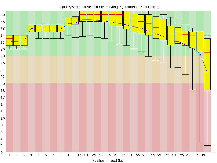
The output is in an HTML file with a graphical representation of various quality metrics. Here is a video explaining the output. Make sure that there is no major problem in your data. Some researchers trim low-quality sequence tails using tools like Trimmomatic. I think that this step was useful in the past, but with the current state of sequence quality, it is not necessary anymore. Moreover, there is evidence that trimming introduces false variants.

Map to the reference genome

GATK Best Practice recommends using BWA aligner for DNA data. BWA is probably the best software in terms of accuracy and speed for mapping sequences with low divergence from a reference. In non-model organisms, the common problem is that the only reference genome available is a sister species that can be considerably divergent. So, one has to use an aligner that accounts for this divergence.

There is a nice blog-post comparing different aligners for mapping divergent sequence reads in Heliconius. As the author of this post, I also prefer to use Stampy. Stampy produces reasonably good results with default settings, however, the accuracy can be improved if the divergence from the reference is correctly specified with option --substitutionrate.

The first step is to prepare the reference genome:

stampy.py -G REF reference_genome.fasta.gz && stampy.py -g REF -H REF

Next, map reads to a reference with account for divergence (0.025 in this case):

stampy.py -t8 -g REF -h REF --substitutionrate=0.025 -o output.sam -M R1.fq.gz R2.fq.gz

See Stampy documentation for details.

If a studied species is too divergent from the closest reference genome available, de novo genome assembly may be a better option. However, mapping to a divergent reference genome usually produces better results than doing rough de novo assembly (ADD reference).

Prepare BAM files

Now, you need to do several steps to prepare BAM files for genotyping with the GATK.

Convert SAM to BAM

The step above produces an alignment in a SAM format. SAM files are tab-delimited text files that are usually very large in size. To save space and make it easy for software to hand large aliments, SAM is usually converted to a binary format BAM. Picard Tools is a recommended software for the conversion as it also allows simultaneous sorting of aligned reads in a file:

java -Xmx8g -jar picard.jar SortSam \
  INPUT=aligned_reads.sam \ 
  OUTPUT=sorted_reads.bam \ 
  SORT_ORDER=coordinate

In some cases Picard Tools fails to perform the conversion. Using SAMtools is an alternative way to proceed then:

samtools view -bS -@ 8 SE14_stampy0.025_DNA.sam > SE14_stampy0.025_DNA.bam
samtools sort -@ 8 SE14_stampy0.025_DNA.bam SE14_stampy0.025_DNA_sorted
samtools index SE14_stampy0.025_DNA_sorted.bam

After BAM files are obtained, SAM files can be deleted. Note! Before deleting any files, make sure that all conversions have been successful. Otherwise, you will have to repeat the mapping step which is quite time-consuming.

Check the mapping quality

Mapping quality can also be assessed on SAM files, but I prefer to analyze BAM files as they are less space consuming. For this analysis, I prefer to use Qualimap. It is reasonably fast and produces very thorough summary with essential graphics.

qualimap bamqc -nt 8 -bam file.bam -outdir results_folder

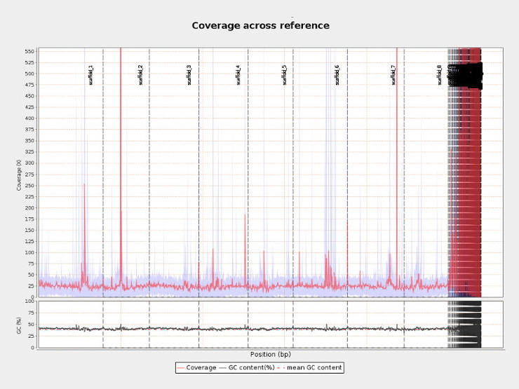
Distributions of coverage, nucleotide content and mapping quality across the reference genome can help to identify problematic regions. For example, in the picture above per-centromeric regions have x100 higher coverage than the rest of the genome and thus interpretation of any finding in these regions should be done with caution.</p>

Mark duplicates

Potential PCR duplicates need to be marked with Picard Tools:

java -Xmx8g -jar picard.jar MarkDuplicates \ 
  INPUT=sorted_reads.bam \ 
  OUTPUT=sorted_reads_duplMarked.bam \
  METRICS_FILE=sorted_reads_duplMarked.metrics \
  MAX_FILE_HANDLES=15000 

MAX_FILE_HANDLES should be little smaller than the output of this command ulimit -n

Marking duplicates make sense even if you used a PCR-free library preparation procedure because reads identified as duplicates are not removed and can be included in the subsequent analyses if needed (GATK option: -drf DuplicateRead).

Add Groups

The GATK requires read group information in BAM files. It is used to differentiate samples and to detect artifacts associated with sequencing techniques. To add read groups, use Picard Tools:

java -Xmx4g -jar picard.jar AddOrReplaceReadGroups \
I=sorted_reads_duplMarked.bam \
O=sorted_reads_duplMarked_readgroup.bam \
RGLB=library \
RGPL=illumina \
RGPU=barcode \
RGSM=sample

Index the resulting BAM file:

samtools index SE14_stampy025_DNA_sorted_DuplMarked_readgroup.bam

Realign Indels

Create a Realigner Target (multi-threading is supported with the -nt option):

java -Xmx4g -jar ~/Programs/GATK/GenomeAnalysisTK.jar \
-T RealignerTargetCreator \
-nt 16 \
-R ~/reference/Crubella_183.fa \
-I sorted_reads_duplMarked_readgroup.bam \
-o sorted_reads_duplMarked_readgroup.intervals \
-log sorted_reads_duplMarked_readgroup.intervals.log

Perform realignment (multi-threading isn't supported):

java -Xmx4g -jar ~/Programs/GATK/GenomeAnalysisTK.jar \
-T IndelRealigner \
-R reference_genome.fasta \
-I sorted_reads_duplMarked_readgroup.bam \
-targetIntervals sorted_reads_duplMarked_readgroup.intervals \
-o sorted_reads_duplMarked_readgroup_realigned.bam

Recalibrate Base Quality Score

The GATK best practices recommend performing Base Quality Score Recalibration. This procedure detects systematic errors in your data by comparing it to the reference training data set. The problem with non-mode organisms is that there is usually no large high confidence genotype database that is required for training.

One of the solutions to this problem is to create a custom training database from the same data you analyze but using very stringent filtering criteria and re-calibrate the data. I addressed this question at the GATK forum and although my approach was supported by the GATK team, in practice it did not work well. It simply shifts the distribution to lower scores as you can see below.

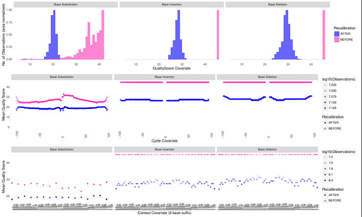
So, unless you have a large training dataset, you probably will have to skip this step.

Genotype

The BAM files ready now and can be processed with the GATK to obtain the genotype data.

Generate GVCF files

Run HaplotypeCaller in GVCF mode on each file:

java -Xmx8g -jar ~/Programs/GATK/GenomeAnalysisTK.jar \
-T HaplotypeCaller \
-nct 16 \
-R reference_genome.fasta \
-I sorted_reads_duplMarked_readgroup_realigned.bam \
-ERC GVCF \
-hets 0.015 \
-indelHeterozygosity 0.01 \
-o sorted_reads_duplMarked_readgroup_realigned.g.vcf

If your study organism is not human, the heterozygosity level may need some adjustment. The default value is 0.001. If your heterozygosity differs specify it with -hets and -indelHeterozygosity. You can estimate it from any previously generated data:

Approximate heterozygosity = ((number of sites with Indels)/(Total number of sites))*(1-(average number of homozygous genotypes per site)/(total number of individuals))

You can calculate the average number of homozygous genotypes per site with this code:

awk -F\0\/0: '!/^ *#/ {total += NF-1; count++} END { print total/count }' Indels.vcf
awk -F\0\/0: '!/^ *#/ {total += NF-1; count++} END { print total/count }' SNPs.vcf

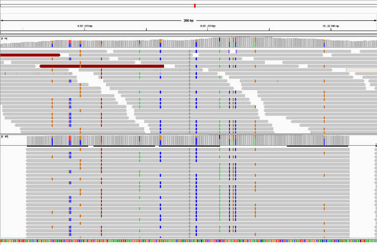
Verify HaplotypeCaller assembly

This is an optional step. HaplotypeCaller performs local reassembly of reads and then genotypes sites. You can produce a BAM file with these localy reassembled fragments and assess the quality in IGV:

java -Xmx8g -jar ~/Programs/GATK/GenomeAnalysisTK.jar \
-T HaplotypeCaller \
-R reference_genome.fasta \
-I sorted_reads_duplMarked_readgroup_realigned.bam \
-ERC GVCF \
-hets 0.015 \
-indelHeterozygosity 0.01 \
-L scaffold_1 \
-bamout sorted_reads_duplMarked_readgroup_realigned_scaffold_1.g.vcf.bam \
-o sorted_reads_duplMarked_readgroup_realigned_scaffold_1.g.vcf

Genotype all GVCF files

Run the GATK on all GVCF files:

java -Xmx8g -jar ~/Programs/GATK/GenomeAnalysisTK.jar \
-T GenotypeGVCFs \
-nt 16 \
-R reference_genome.fasta \
-V 01_sorted_reads_duplMarked_readgroup_realigned.g.vcf \
-V 02_sorted_reads_duplMarked_readgroup_realigned.g.vcf \
-V 03_sorted_reads_duplMarked_readgroup_realigned.g.vcf \
-V 04_sorted_reads_duplMarked_readgroup_realigned.g.vcf \
-V 05_sorted_reads_duplMarked_readgroup_realigned.g.vcf \
-V 06_sorted_reads_duplMarked_readgroup_realigned.g.vcf \
-V 07_sorted_reads_duplMarked_readgroup_realigned.g.vcf \
-V 08_sorted_reads_duplMarked_readgroup_realigned.g.vcf \
-V 09_sorted_reads_duplMarked_readgroup_realigned.g.vcf \
-V 10_sorted_reads_duplMarked_readgroup_realigned.g.vcf \
-hets 0.015 \
-indelHeterozygosity 0.01 \
-stand_call_conf 30.0 \
-allSites \
-o GVCFall.vcf

You can adjust -stand_call_conf or add any other filers depending on your needs.

Also, I usually genotype all sites (i.e. non-variable and polymorphic) with the option -allSite and select variable sites later. It is necessary because estimation of some population genetics statistics require scaling by a total number of sites (i.e. including non-variable).

Select SNPs and Indels

Select SNPs:

java -Xmx8g -jar ~/Programs/GATK/GenomeAnalysisTK.jar \
-T SelectVariants \
-R reference_genome.fasta \
-V GVCFall.vcf \
-selectType SNP \
-o GVCFall_SNPs.vcf

Select Indels:

java -Xmx8g -jar ~/Programs/GATK/GenomeAnalysisTK.jar \
-T SelectVariants \
-R reference_genome.fasta \
-V GVCFall.vcf \
-selectType INDEL \
-o GVCFall_INDELs.vcf

Filter Variants

I first perform filtering of variant sites and then filter individual genotypes.

Variants filtering is applied to SNPs/Indels VCF files only, whereas genotype filtering can be applied to both SNPs/Indels VCFs and whole genome VCFs.

Extract Variant Quality Scores

For SNPs:

java -jar ~/Programs/GATK/GenomeAnalysisTK.jar \
-T VariantsToTable \
-R reference_genome.fasta \
-V GVCFall_SNPs.vcf \
-F CHROM -F POS -F QUAL -F QD -F DP -F MQ -F MQRankSum -F FS -F ReadPosRankSum -F SOR \
--allowMissingData \
-o GVCFall_SNPs.table

For Indels:

java -jar ~/Programs/GATK/GenomeAnalysisTK.jar \
-T VariantsToTable \
-R reference_genome.fasta \
-V GVCFall_INDELs.vcf \
-F CHROM -F POS -F QUAL -F QD -F DP -F MQ -F MQRankSum -F FS -F ReadPosRankSum -F SOR \
--allowMissingData \
-o GVCFall_INDELs.table

These scores will be used to build distributions and define filtering cutoffs.

Make diagnostic plots for Variants Scores

Run this R code:

library('gridExtra')
library('ggplot2')

VCFsnps <- read.csv('GVCFall_SNPs.table', header = T, na.strings=c("","NA"), sep = "\t") 
VCFindel <- read.csv('GVCFall_INDELs.table', header = T, na.strings=c("","NA"), sep = "\t")
dim(VCFsnps)
dim(VCFindel)
VCF <- rbind(VCFsnps, VCFindel)
VCF$Variant <- factor(c(rep("SNPs", dim(VCFsnps)[1]), rep("Indels", dim(VCFindel)[1])))

snps <- '#A9E2E4'
indels <- '#F4CCCA'

DP <- ggplot(VCF, aes(x=DP, fill=Variant)) + geom_density(alpha=0.3) + 
  geom_vline(xintercept=c(10,6200))

QD <- ggplot(VCF, aes(x=QD, fill=Variant)) + geom_density(alpha=.3) +
  geom_vline(xintercept=2, size=0.7)

FS <- ggplot(VCF, aes(x=FS, fill=Variant)) + geom_density(alpha=.3) +
  geom_vline(xintercept=c(60, 200), size=0.7) + ylim(0,0.1)

MQ <- ggplot(VCF, aes(x=MQ, fill=Variant)) + geom_density(alpha=.3) +
  geom_vline(xintercept=40, size=0.7)

MQRankSum <- ggplot(VCF, aes(x=MQRankSum, fill=Variant)) + geom_density(alpha=.3) +
  geom_vline(xintercept=-20, size=0.7)

SOR <- ggplot(VCF, aes(x=SOR, fill=Variant)) + geom_density(alpha=.3) +
  geom_vline(xintercept=c(4, 10), size=1, colour = c(snps,indels))

ReadPosRankSum <- ggplot(VCF, aes(x=ReadPosRankSum, fill=Variant)) + geom_density(alpha=.3) +
  geom_vline(xintercept=c(-10,10,-20,20), size=1, colour = c(snps,snps,indels,indels)) + xlim(-30, 30)

svg("Co_10accessions_FromStephen.svg", height=20, width=15)
theme_set(theme_gray(base_size = 18))
grid.arrange(QD, DP, FS, MQ, MQRankSum, SOR, ReadPosRankSum, nrow=4)
dev.off()

It will produce these plots:

Annotations: DP - combined depth per SNP across samples (24 samples in the case above) QD - variant confidence standardized by depth. MQ - Mapping quality of a SNP. FS - strand bias in support for REF vs ALT allele calls SOR - sequencing bias in which one DNA strand is favored over the other MQRankSum - Rank sum test for mapping qualities of REF vs. ALT reads. ReadPosRankSum - do all the reads support a SNP call tend to be near the end of a read.

Apply Variant filtering

I filter the data following the GATK best practice with some adjustment for my data. For example, I relax MQRankSum filter because in my case reads are more divergent from the reference than expected. I define cutoffs based on the distribution of a particular score to keep as much data as possible but also remove the least confident sites.

To filter SNPs:

java -jar ~/Programs/GATK/GenomeAnalysisTK.jar \
 -T VariantFiltration \
 -R reference_genome.fasta \
 -V GVCFall_SNPs.vcf \
 --filterExpression "QUAL < 0 || MQ < 30.00 || SOR > 4.000 || QD < 2.00 || FS > 60.000 || MQRankSum < -20.000 || ReadPosRankSum < -10.000 || ReadPosRankSum > 10.000" \ # you define what to remove here
 --filterName "my_snp_filter" \
 -o GVCFall_SNPs_filter.vcf

grep -E '^#|PASS' GVCFall_SNPs_filter.vcf > GVCFall_SNPs_filterPASSED.vcf

To filter Indels:

java -jar ~/Programs/GATK/GenomeAnalysisTK.jar \
 -T VariantFiltration \
 -R reference_genome.fasta \
 -V GVCFall_INDELs.vcf \
 --filterExpression "QUAL < 0 || MQ < 30.00 || SOR > 10.000 || QD < 2.00 || FS > 200.000 || ReadPosRankSum < -20.000 || ReadPosRankSum > 20.000" \ # you define what to remove here
 --filterName "my_indel_filter" \  
 -o GVCFall_INDELs_filter.vcf

grep -E '^#|PASS' GVCFall_INDELs_filter.vcf > GVCFall_INDELs_filterPASSED.vcf

Check the Variants filtering results

I look at how many sites have been removed.

This is the number of sites before filtering:

grep -vc "^#" GVCFall_INDELs.vcf
grep -vc "^#" GVCFall_SNPs.vcf

This is the number of sites retained after filtering:

grep -vc "^#" GVCFall_SNPs_filterPASSED.vcf
grep -vc "^#" GVCFall_INDELs_filterPASSED.vcf

It is also important to check if any filers failed. I observed filters failing often. Generate scores table for filtered data as in the step "Extract Quality Scores" above. You should get 0 for all filters when you run this R code:

# SNPs
VCFsnps <- read.csv('GVCFall_SNPs_filterPASSED.table', header = T, na.strings=c("","NA"), sep = "\t") 
head(VCFsnps)
sum(na.omit(VCFsnps$QD) < 2)
sum(na.omit(VCFsnps$FS) > 60)
sum(na.omit(VCFsnps$MQ) < 40)
sum(na.omit(VCFsnps$MQRankSum) < -20)
sum(na.omit(VCFsnps$SOR) > 4)
sum(na.omit(VCFsnps$ReadPosRankSum) < -10)
sum(na.omit(VCFsnps$ReadPosRankSum) > 10)

 # Indels
VCFindel <- read.csv('GVCFall_INDELs_filterPASSED.table', header = T, na.strings=c("","NA"), sep = "\t")
head(VCFindel30)
sum(na.omit(VCFindel$QD) < 2)
sum(na.omit(VCFindel$FS) > 200)
sum(na.omit(VCFindel$MQ) < 40)
sum(na.omit(VCFindel$SOR) > 10)
sum(na.omit(VCFindel$ReadPosRankSum) < -20)
sum(na.omit(VCFindel$ReadPosRankSum) > 20)

If some of the filters failed, try to change their order in --filterExpression.

Filter genotypes

When all low confidence variant sites are removed, I filer VCF files for genotype quality. GATK provides several annotation scores for genotypes, but they cannot be used equally for variant and non-variant sites (e.g. GQ in SNPs and RGQ in non-variant sites). It is not reasonable to filter such scores simultaneously because this will introduce bias to variant/non-variant sites ratio. So, I usually filter only by depth (Note, the genotype quality filter of 30 has been also applied during GenotypeGVCFs calling.).

Extract depth information

I usually assess this information only for the whole genome VCF.

java -Xmx8g -jar ~/Programs/GATK/GenomeAnalysisTK.jar \
 -T VariantsToTable \
 -R reference_genome.fasta \
 -V GVCFall.vcf \
 -F CHROM -F POS -GF GT -GF DP \
 -o GVCFall.DP.table

Visualize the extracted information

The file GVCFall.DP.table is usually too big for R, so I split it by samples and keep only positions that have been genotyped (!="./."):

for ((i=3; i<=21; i +=2)); do cut -f $i,$((i+1)) GVCFall.DP.table | awk '$1 != "./." {print $2}' > $i.DP; done

where 3-21 is odd numbers for 10 samples. This numbering is required because every sample is represented by two columns (GT, DP).

Plot DP distribution and define cut-off (edit number for your sample size):

# define the file names list (10 samples here) 
nameList <- c()
for (i in 3:21) { # 21 - odd number for 10 samples 
  if (i %% 2 ==1) nameList <- append(nameList, paste(i, ".DP"))
}

qlist <- matrix(nrow = 10, ncol = 3) # define number of samples (10 samples here)
qlist <- data.frame(qlist, row.names=nameList)
colnames(qlist)<-c('5%', '10%', '99%')

jpeg("GVCFall.DP.jpeg", height=1600, width=1200)
par(mar=c(5, 3, 3, 2), cex=1.5, mfrow=c(8,4)) # define number of plots for your sample
for (i in 1:31) {
  DP <- read.table(nameList[i], header = T)
  qlist[i,] <- quantile(DP[,1], c(.05, .1, .99), na.rm=T)
  d <- density(DP[,1], from=0, to=100, bw=1, na.rm =T)
  plot(d, xlim = c(0,100), main=nameList[i], col="blue", xlab = dim(DP)[1], lwd=2)
  abline(v=qlist[i,c(1,3)], col='red', lwd=3)
}
dev.off()

write.table(qlist, "GVCFall.DP.percentiles.txt")

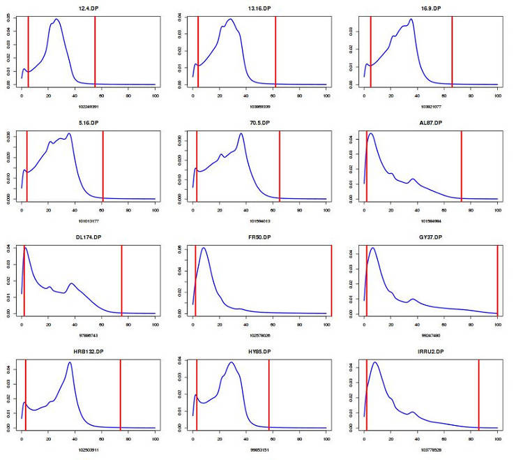
You can view the content of GVCFall.DP.percentiles.txt and select the acceptable cut-off. I usually discard the genotypes below the 5th percentile and above the 99th percentile.

Apply depth filter

Mark filtered genotypes:

java -jar ~/Programs/GATK/GenomeAnalysisTK.jar \
 -T VariantFiltration \
 -R reference_genome.fasta \
 -V GVCFall.vcf \
 -G_filter "DP < 6 || DP > 100" \
 -G_filterName "DP_6-100" \
 -o GVCFall_DPfilter.vcf

java -jar ~/Programs/GATK/GenomeAnalysisTK.jar \
 -T VariantFiltration \
 -R reference_genome.fasta \
 -V GVCFall_SNPs_filterPASSED \
 -G_filter "DP < 6 || DP > 100" \
 -G_filterName "DP_6-100" \
 -o GVCFall_SNPs_filterPASSED_DPfilter.vcf

java -jar ~/Programs/GATK/GenomeAnalysisTK.jar \
 -T VariantFiltration \
 -R reference_genome.fasta \
 -V GVCFall_Indels_filterPASSED.vcf \
 -G_filter "DP < 6 || DP > 100" \
 -G_filterName "DP_6-100" \
 -o GVCFall_Indels_filterPASSED_DPfilter.vcf

Set filtered sites to no call:

java -jar ~/Programs/GATK/GenomeAnalysisTK.jar \
 -T SelectVariants \
 -R reference_genome.fasta \
 -V GVCFall_DPfilter.vcf \
 --setFilteredGtToNocall \
 -o GVCFall_DPfilterNoCall.vcf

java -jar ~/Programs/GATK/GenomeAnalysisTK.jar \
 -T SelectVariants \
 -R reference_genome.fasta \
 -V GVCFall_SNPs_filterPASSED_DPfilter.vcf \
 --setFilteredGtToNocall \
 -o GVCFall_SNPs_filterPASSED_DPfilterNoCall.vcf

java -jar ~/Programs/GATK/GenomeAnalysisTK.jar \
 -T SelectVariants \
 -R reference_genome.fasta \
 -V GVCFall_Indels_filterPASSED_DPfilter.vcf \
 --setFilteredGtToNocall \
 -o GVCFall_Indels_filterPASSED_DPfilterNoCall.vcf

VCF to Tab

When all filters have been applied, I do not need the annotation information any more, so I only keep the high confidence genotypes:

java -Xmx8g -jar ~/Programs/GATK/GenomeAnalysisTK.jar \
 -T VariantsToTable \
 -R reference_genome.fasta \
 -V GVCFall_DPfilterNoCall.vcf \
 -F CHROM -F POS -GF GT \
 -o whole_Genome.table

java -Xmx8g -jar ~/Programs/GATK/GenomeAnalysisTK.jar \
 -T VariantsToTable \
 -R reference_genome.fasta \
 -V GVCFall_SNPs_filterPASSED_DPfilterNoCall.vcf \
 -F CHROM -F POS -GF GT \
 -o SNPs.table

java -Xmx8g -jar ~/Programs/GATK/GenomeAnalysisTK.jar \
 -T VariantsToTable \
 -R reference_genome.fasta \
 -V GVCFall_Indels_filterPASSED_DPfilterNoCall.vcf \
 -F CHROM -F POS -GF GT \
 -o Indels.table

I also usually convert two-character coded to single-character coded genotypes. More details here.

python vcfTab_to_callsTab.py -i whole_Genome.table -o whole_Genome.tab
python vcfTab_to_callsTab.py -i SNPs.table -o SNPs.tab

Merge the whole genome and SNPs files (optional)

Depending on your analyses, you may also want to merge SNPs and whole genome files. These two files were filtered differently, with more stringency on SNP file. So, some of the genotypes in the whole genome file are more likely to be false positives. To eliminate such genotypes, you can remove polymorphic sites in the whole genome file if they are not present in the SNPs file. This can be done with my merge_SNP_wholeGenome_TabFiles.py script. Note, you first need to convert two-character coded genotypes to single-character coded genotypes as I have just mentioned above:

python merge_SNP_wholeGenome_TabFiles.py -g whole_Genome.tab -s SNPs.tab -o merged.tab

What is next?

Now, it is very easy to write custom scripts to convert these genotype tables to any other format or analyze them directly.

You can find many scripts to process such tab-delimited genotype calls in my GitHub repository.

If you have any questions or suggestions, feel free to email me.