Interpopulation comparison of Copy Number Variants
Guide on how to process Copy Number Variants generated with GATK 4 to compare samples from different populations
I showed how to efficiently genotype Copy Number Variants with GATK and Snakemake. As a continuation of the Copy Number Variation topic, I will share how I compared the Copy Number Variation along the genome between three different populations. If you also analyze the population genomic data, I hope you will find this post useful.
Although the GATK Copy Number Variants (CNVs) calling pipeline utilizes the population variation during the CNVs calling in the cohort mode, it produces separate VCF files for each sample. The CNVs in such VCF files look similar to this:
#CHROM  POS     ID      REF     ALT     QUAL    FILTER  INFO    FORMAT  sample1
chrN    45894001        CNV_45894001_46949000      N       <DEL>,<DUP>     .       .       END=46949000    GT:CN:NP:QA:QS:QSE:QSS  0:2:1055:47:3077:78:119
chrN    46949001        CNV_46949001_46956000      N       <DEL>,<DUP>     .       .       END=46956000    GT:CN:NP:QA:QS:QSE:QSS  2:4:7:6:9:15:8
chrN    46956001        CNV_46956001_55222000      N       <DEL>,<DUP>     .       .       END=55222000    GT:CN:NP:QA:QS:QSE:QSS  0:2:8263:17:3077:108:19
chrN    55222001        CNV_55222001_55223000      N       <DEL>,<DUP>     .       .       END=55223000    GT:CN:NP:QA:QS:QSE:QSS  1:0:1:493:493:493:493
If you compare the CNVs from different samples, most likely you will find that breaking points are not the same across your samples. This poses a problem of connecting the CNVs from different samples to estimate the interpopulation differences along the genome.
To overcome this problem, we decided to bin each CNV segments according to breaking points it overlaps. This allowed us to merge CNVs of all samples into one large table where the genomic coordinates are the same:
CHROM	 POS	     END       s1   s2  s3  s4  s5  s6  s7  s8
chrN	46939001	46949000	2	2	2	2	2	2	2	2
chrN	46949001	46951000	4	5	1	4	5	1	4	3
chrN	46951001	46955000	4	5	1	4	5	1	4	3
chrN	46955001	46956000	4	5	1	4	5	1	4	3
chrN	46956001	46957000	2	2	2	2	2	2	2	2
Such a table can be used to estimate various statistics along the genome for different populations. For example, I estimated Vst between populations (it’s like Fst but for CNVs.)
Let me show you everything step-by-step.
Visualize the CNV variation
To make sure my CNV calls are good, I explored the CNV variation between my samples in IGV.
First, I extracted the CNV genotypes form the VCF files using GATK and converted the resulting tables into seg and tab formats using Snakemake:
# Use Snakemake 4, GATK 4

CHROMOSOMES, SAMPLES, = glob_wildcards('chr{i}_{sample}_segments_cohort.vcf')
REF = '/path/to/reference.fa'

rule all:
    input:
        expand('chr{i}_{sample}_segments_cohort.seg', sample=SAMPLES, i=CHROMOSOMES)

rule toTable:
    input:
        ref = REF,
        vcf = 'chr{i}_{sample}_segments_cohort.vcf'
    output:
       'chr{i}_{sample}_segments_cohort.table'
    shell:
        '''
        gatk --java-options "-Xmx8G" VariantsToTable \
        -R  {input.ref} \
        -V  {input.vcf} \
        -F ID -GF CN \
        -O {output}
        '''

rule toSeg:
    input:
        'chr{i}_{sample}_segments_cohort.table'
    output:
       seg = 'chr{i}_{sample}_segments_cohort.seg',
       tab = 'chr{i}_{sample}_segments_cohort.tab'
    params:
        '{sample}'
    shell:
        '''
        sed 's/CNV_//g;s/_/\t/g' {input} | \
        awk -v s={params} 'BEGIN{ {print "CHROM\\tPOS\\tEND\\t"s".CN"} } NR>1 { {print $0} }' \
        >  {output.tab} && \
        sed 's/CNV_//g;s/_/\t/g' {input} | \
        awk -v s={params} 'BEGIN{ { print s"\\tCHROM\\tPOS\\tEND\\t"s".CN" } } NR>1 { {print s"\\t"$0} }' \
        >  {output.seg}
        '''
This produced three files per sample. Here is the example of these files:
chrN_sample1_segments_cohort.table:
ID                              sample1.CN
CNV_chrN_45894001_46949000        2
CNV_chrN_46949001_46956000        4
CNV_chrN_46956001_55222000        2
CNV_chrN_55222001_55223000        0
chrN_sample1_segments_cohort.tab:
CHROM   POS     END     sample1.CN
chrN    45894001        46949000        2
chrN    46949001        46956000        4
chrN    46956001        55222000        2
chrN    55222001        55223000        0
chrN_sample1_segments_cohort.seg:
sample1        CHROM     POS            END     sample1.CN
CFA010182       chrN    45894001        46949000        2
CFA010182       chrN    46949001        46956000        4
CFA010182       chrN    46956001        55222000        2
CFA010182       chrN    55222001        55223000        0
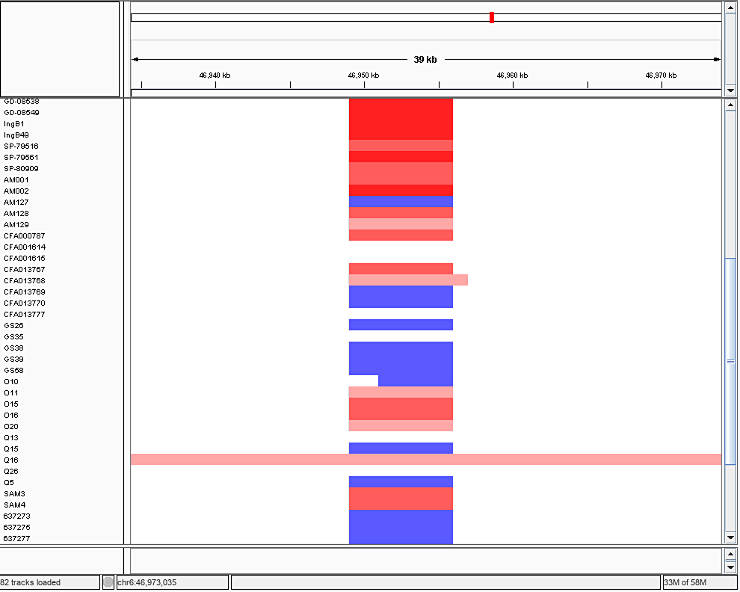
Then, you load the *.seg files into IGV and you will obtain a picture similar to this one:
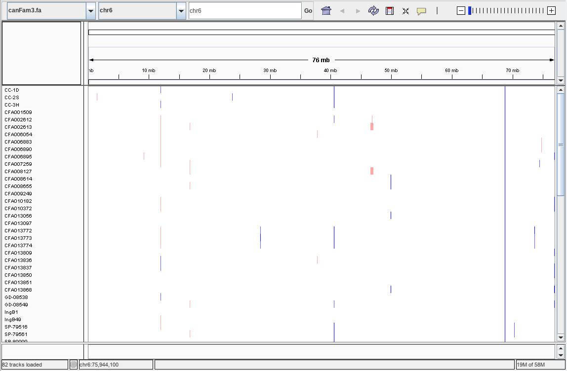
In IGV, read indicates duplications, blue marks deletions, and white depicts the diploid state. The intensity of the color corresponds to number of gained or lost copies.
Bin the segments
To bin all the segments into the same set of segments across samples, I merged and sorted the coordinates from all samples:
cat chrN_*_segments_cohort.tab | cut -f 1,2,3 | grep -v POS | sort -V -u -k 2,2 -k 3,3 | awk 'BEGIN{print"CHROM\tPOS\tEND"}{print $0}' > CNV_intervals.bed
And created the reference interval file in R:
d <- read.table('chrN_CNV_intervals.bed', header = T)

breaks <- sort(unique(c(d$POS-1, d$END)))
bins <- data.frame(CHROM=rep('chrN', length(breaks[-1])), POS = head(breaks, -1)+1, END=breaks[-1])
options(scipen = 999) # disables scientific notation
write.table(bins, 'CNV_intervals_bins.bed', sep='\t', quote = F, row.names = F)
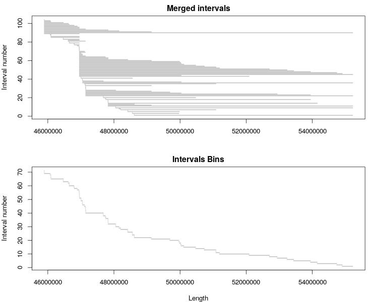
You can visualize the original interval list and bins with this R code:
plot_intervals <- function(df) {
  lines <- c(1:length(df$CHROM))
  nLines <- max(lines)
  plot(0, xlim = c(min(df$POS), max(df$END)), ylim = c(1, nLines), type="n",
       main = "Merged intervals", xlab="", ylab="Interval number")
  for (i in lines){
    segments(df$END[i], nLines+1-i, df$POS[i], nLines+1-i, lwd=2, col = "gray")
  }
}

jpeg('chrN_CNV_intervals_bins.jpeg', width = 740, height = 600)
par(mar=c(4,4,2,1), mfrow=c(2,1), cex=1.1)
plot_intervals(d)
plot_intervals(bins)
dev.off()
Merge all CNV files
Then, I used merge_CNVs_tabs.py to merge all CNV files with CNV_intervals_bins.bed:
for i in *_segments_cohort.tab
    do
        python ~/git/genotype-files-manipulations/merge_CNVs_tabs.py -i $i -r chrN_CNV_intervals_bins.bed -o $i.bin && cut -f 4 $i.bin > $i.bin.col4
    done
paste sample1_segments_cohort.tab.bin tab/*.bin.col4 > segments_cohort_bins.tab
The resulting files have the following format:
CHROM	 POS	     END       s1   s2  s3  s4  s5  s6  s7  s8
chrN	46939001	46949000	2	2	2	2	2	2	2	2
chrN	46949001	46951000	4	5	1	4	5	1	4	3
chrN	46951001	46955000	4	5	1	4	5	1	4	3
chrN	46955001	46956000	4	5	1	4	5	1	4	3
chrN	46956001	46957000	2	2	2	2	2	2	2	2
Calculate Vst
The obtained segments_cohort_bins.tab can be used to calculate various statistics. For example, you can calculate Vst in R:
d <- read.table('chrN_segments_cohort_bins.tab', header = T)

dd <- d[,-c(1:3)]
group <- factor(c("red", "black", "blue", "red", "black", "blue", "red", "blue"))

getVst <- function(dat, groups, comparison) {
  groupLevels <- levels(groups)
  dat1 <- na.omit(dat[groups==groupLevels[groupLevels==comparison[1]]])
  dat2 <- na.omit(dat[groups==groupLevels[groupLevels==comparison[2]]])
  Vtotal <- var(c(dat1, dat2))
  Vgroup <- ((var(dat1)*length(dat1)) + (var(dat2)*length(dat2))) /
             (length(dat1)+length(dat2))
  Vst <- c((Vtotal-Vgroup) / Vtotal)
  if (Vst == "NaN"){
    Vst <- 0
  }
  return(Vst)
}

d$Vst_red_black <- apply(dd, 1, function(x) getVst(x, group, c("red", "black")))
d$Vst_red_blue <- apply(dd, 1, function(x) getVst(x, group, c("red", "blue")))
d$Vst_blue_black <- apply(dd, 1, function(x) getVst(x, group, c("blue", "black")))

write.table(d, 'chrN_segments_cohort_bins_Vst.csv', sep='\t', quote = F, row.names = F)
The table segments_cohort_bins_Vst.csv will look like this:
CHROM   POS    END     s1 s2 s3 s4 s5 s6 s7 s8 Vst_red_black Vst_red_blue Vst_blue_black
chrN 46939001 46949000  2  2  2  2  2  2  2  2             0    0.0000000            0.0
chrN 46949001 46951000  4  5  1  4  5  1  4  3             1    0.6923077            0.8
chrN 46951001 46955000  4  5  1  4  5  1  4  3             1    0.6923077            0.8
chrN 46955001 46956000  4  5  1  4  5  1  4  3             1    0.6923077            0.8
chrN 46956001 46957000  2  2  2  2  2  2  2  2             0    0.0000000            0.0
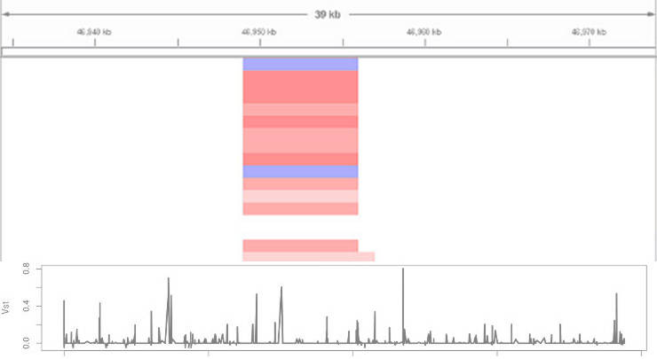
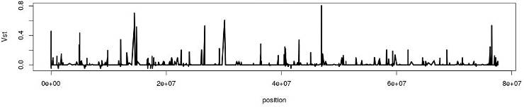
Exploring the distribution of Vst can identify genomic regions of hight divergence:
Final thought
You can use the CNV table chrN_segments_cohort_bins.tab to calculate many other things.
We found to be the most parsimonious solution to bin the CNV segments to merge all samples into one table. If there is a better way to solve the problem of variation in breaking points of CNVs for the interpopulation comparison, please let me know.
If you have any questions or suggestions, feel free to email me.